L-Py Editor¶

First look on the editor¶

L-Py has a built-in editor developped with Qt, an UI-designed library.

On start, the editor looks like this:

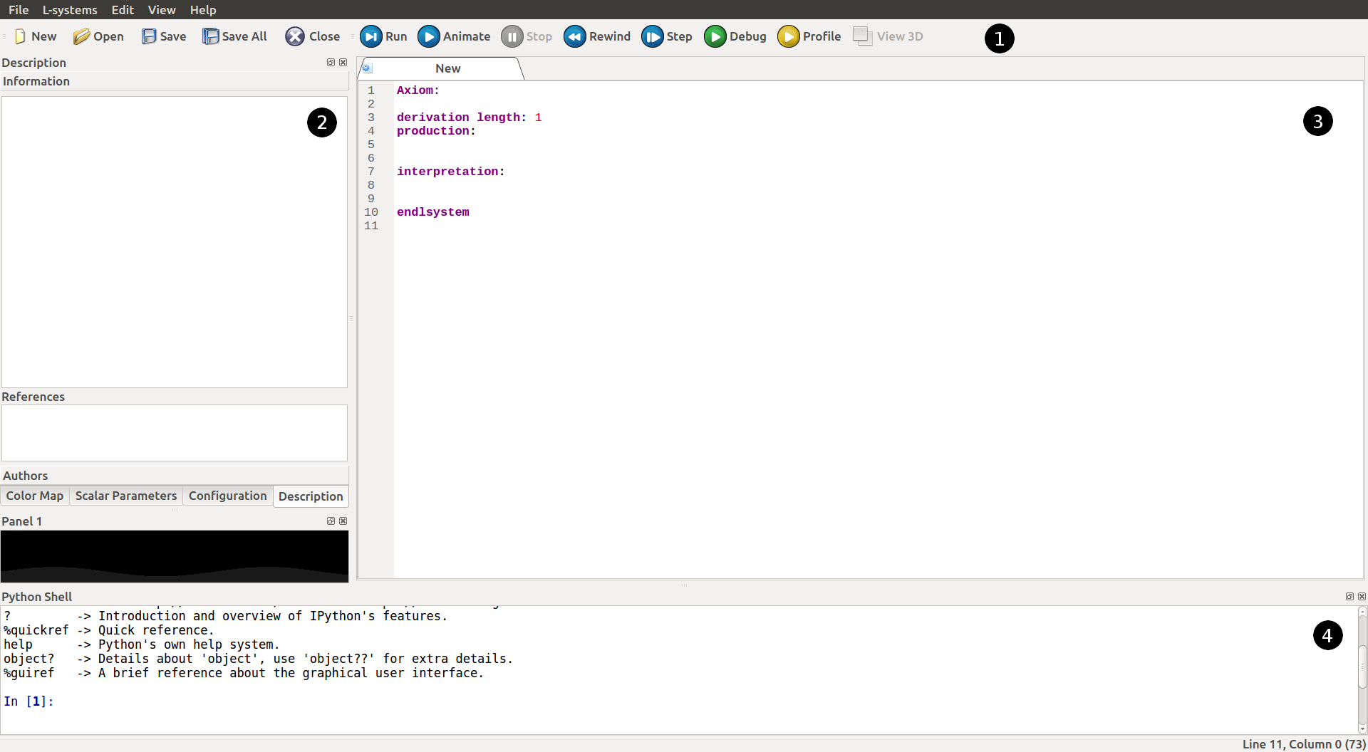
1) Top Toolbar

This toolbar present the most used features of L-Py. You can create, open or save your current program; you can run and animate your work with the appropriate buttons or even execute it step by step and ultimately you can debug or check the process and rendering time with the Profile button.

2) Sidebar tools

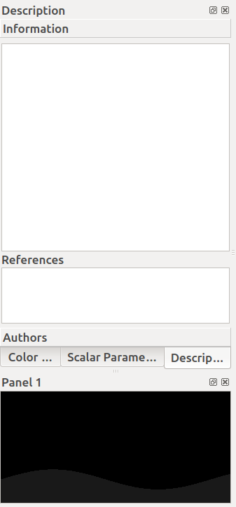
On the left sidebar, meta information on the model and its execution can be defined or controlled :

“Color map” : Creation of custom materials or textures to assign to objects of the simulation.
“Configuration” : Configure the settings of the execution of the model.
“Description” : Presentation of the models and its contributors.

3) Editor

L-Py gives you the possibility to code inside the application by a built-in editor. All L-Py keywords are recognized and colored for a best readability.

4) Python Shell

A Python Shell makes it possible to manipulates the lsystems and theirs variables.

5) Custom panels

Some panels for the definition of graphical object such as function, curves of patches.

PlantGL Viewer¶

By default, the visualization of the model is made within the PlantGL Viewer after clicking on Run or Animate buttons .

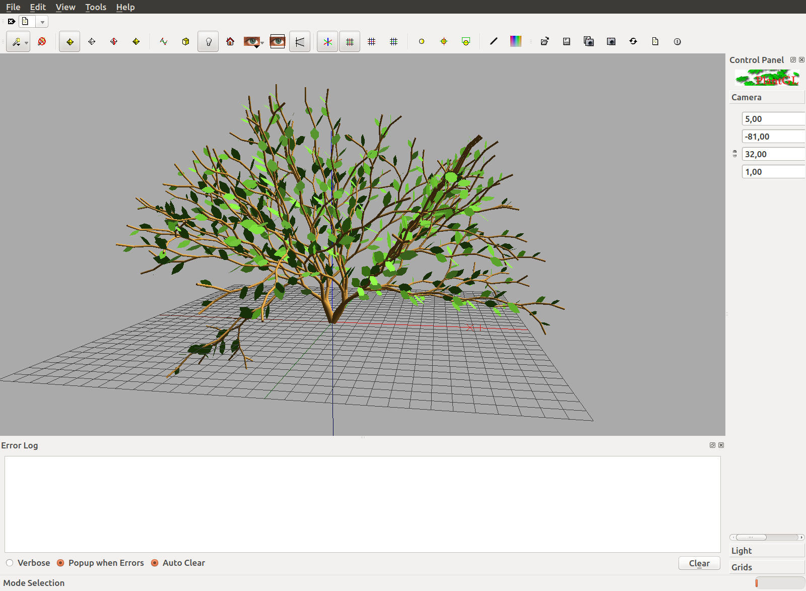
The PlantGL visualizer has a 3D-camera where you can turn around your object. The basic controls you’ll mostly use are:

Hold Left Click to turn around X and the Y axis of the camera
Wheel Mouse to zoom / unzoom on the scene
Hold Right Click to shift the scene on the screen

Color Map¶

It can be used to create colors and access it directly in your code by avoiding multiple duplications of SetColor(r,g,b[,a]) thanks to the ‘,’ ‘;’ or SetColor(index) instructions.

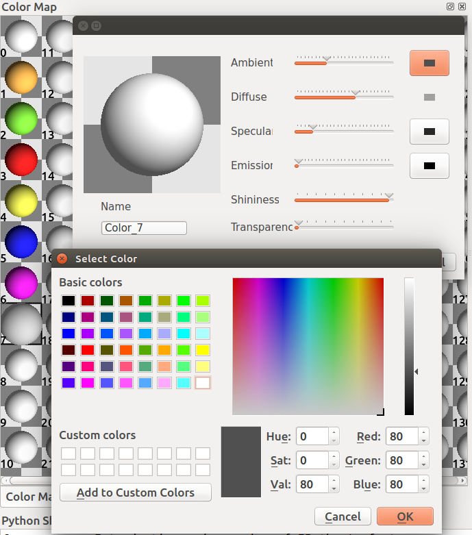
When double-clicking on a material sphere, a dialog appears to configure a custom material.

The ambient, diffuse, specular, emission, shininess and transparency components of the material can be controled.

Scalar Parameters¶

A model may have critical parameters whose values need to be controled finelly. For this some graphical control are possible using the Scalar Parameters sidebar. In this bar, you can create a scalar parameter by defining a name, a type (bool, integer, float), some bounds. The name of the parameter will correspond to the name of the variable that will be created within the model.

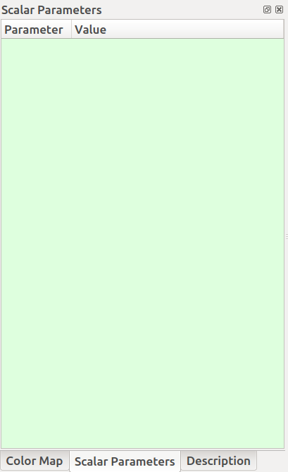
First, a right-click in the green area makes it possible to create a new scalar parameter. A definition dialog pops up.

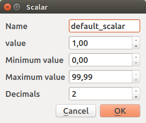
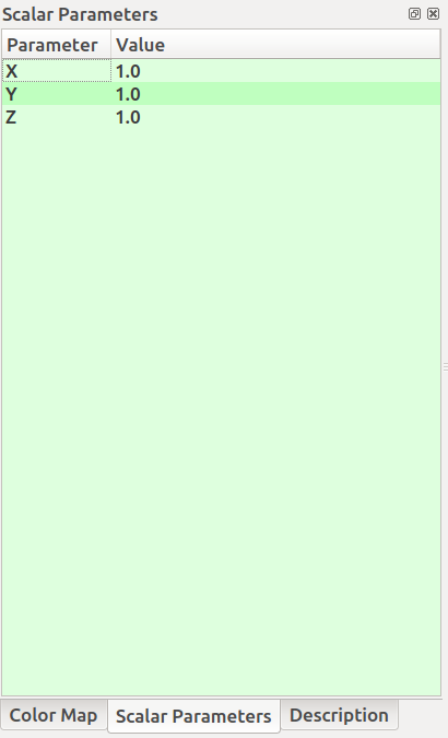
As a result different variables can be added and are accessible in the toolbar.

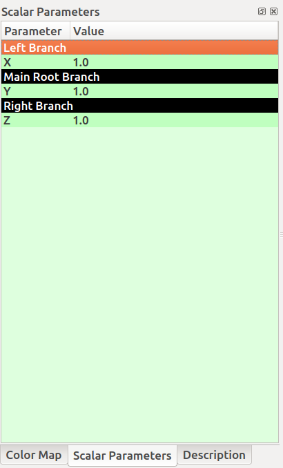
To organize these variables, some categories can be added, represented in black.

Code:

Within the code, the variables can be used as standard variables. In the following example, the previous X,Y, Z parameters are used as value of length of different branch of a simple structure.

Axiom: B[+A][-F(Z)]

production:

interpretation:
A --> F(X)
B --> F(Y)

endlsystem

Then, with the code above, double left-click on the values at the right, play with the slider that appeared and click on Run or Animate.

The render on PlantGL should display something like this (with X=4, Y=2 and Z=1.5):

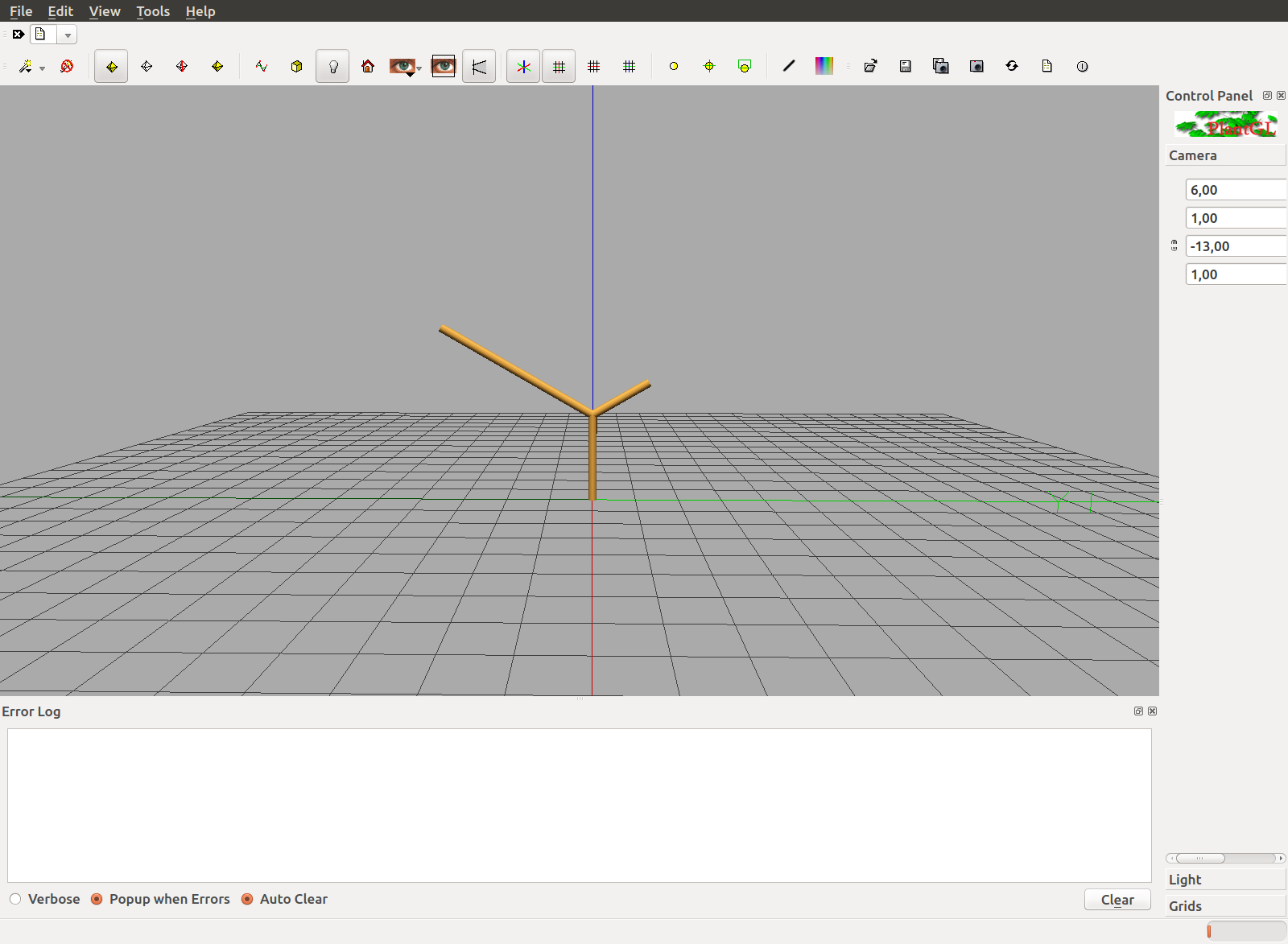
The values put on in the Scalar Parameters widget are directly modified into the code and then displayed on screen on request.

To avoid modifying the values and clicking each time on the Run button, ythe Auto-Run feature can be activated in the menu L-systems > Auto-Run. Every modificaiton of the value will relaunch automatically the simulation.

Custom Curves¶

Enable the Curve Panel¶

First of all, you need to display the widget Panel 1. To do this, right click on an empty space in the top toolbar and click on Panel 1 if it’s disabled.

The panel is usually located below the Sidebar Tools:

but you can drag this widget anywhere you want in the window for your needs.

Create a Bezier curve¶

To create a custom curve, just right-click in the black panel and select “New item > Curve2D > BezierCurve”

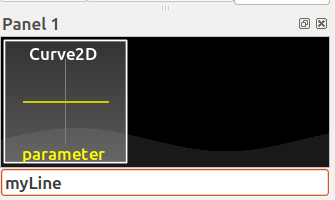
A line edit appears at the bottom of the panel to name your curve and confirm it with Enter. You can rename your curve anytime by right-cliking on the curve component and on “Rename”.

Configure a curve component¶

When double left-clicking on your curve component, a new pop-up appears and shows:

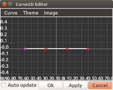
In this interface you can:

Hold Left Click on a dot and drag it to change the curvature of the curve
Double Left Click to create a new checkpoint for the curve
Double Right Click on a dot to delete the selected checkpoint
Wheel Mouse to zoom / unzoom in the interface
Hold Left Click in the black area to shift the curve on the screen

Exemple:

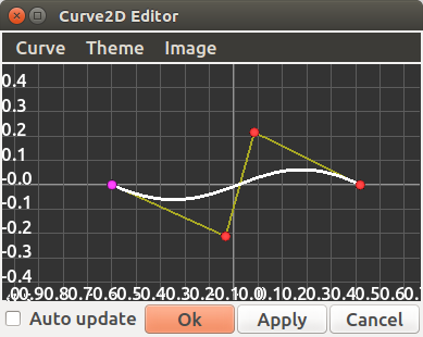
When you’re satisfied with your curve configuration, you can click on the Apply button and close the pop-up.

Debugger¶

As you may know, the render of your project is done with PlantGL. The fact is that L-Py keep as a string your project and, thanks to the string, convert it into instructions to PlantGL.

With the debugger, you can see step by step what is contained in that string and check what’s going, to do so, click on the Debug button in the top toolbar.

You’ll see a new tab “Debugger” opened at the bottom of L-Py:

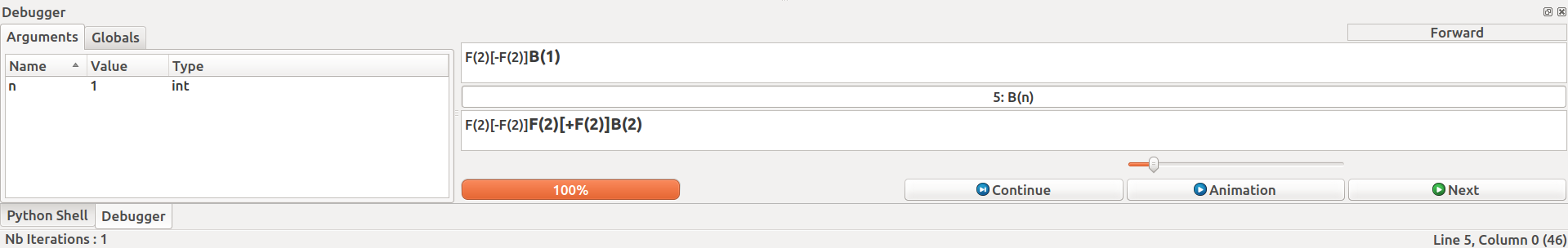
At the top, you can see the string representing your project at the beginning of the current step and below, the string being transformed into by the rules of your project.

The exemple above can be tested with that code:

Axiom: B(0)
derivation length: 4

production:

B(n):
    if (n % 2):
        produce F(2)[+F(2)]B(n + 1)
    else:
        produce F(2)[-F(2)]B(n + 1)

endlsystem

and at the step 2 of the debug mode.

Profiler¶

The profiler is a widget that can help you to see how much time is being spent in each part of your program. It can be very useful into optimizing your project by fixing some parts of your program.

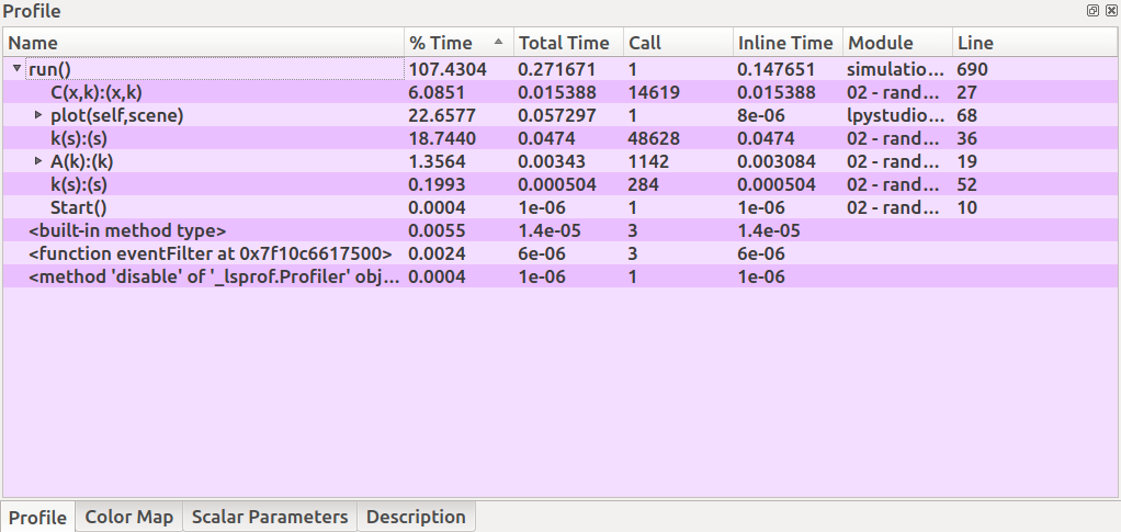
This is sorted as:

Name : The name of the function
% Time : The task time spent divided by the full time spent multiplied by 100
Call : How much time this function has been called
Inline time
Module : In which module the function has been called
Line : Where does the function start in its module

The run() function is basically the entire process, but you can find all your rules in this run() function plus the plot() function, which is the scene rendering function by PlantGL.

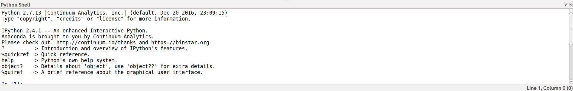
Python Shell¶

You can find at the bottom of L-Py a Python Shell that can be useful to display at run-time some data from your project. The Python Shell implemented looks familiar to a simple shell if you’re used to a Linux or Mac System:

You can find in the Lpy Helpcard all of the available commands for the Python Shell. Here will be explained all known commands at this date:

lstring¶

When lstring is called, this command write on the shell the last computed lsystem string of the current simulation.

Do you remember the Scalar Parameters exemple ? Try to get it again and try to send the lstring command in the Python Shell, you should have this being returned:

In [1]: lstring
Out[1]: AxialTree(B[+A][-F(1.5)])

We can see that, here, the code has been interpreted as an AxialTree, which is the system module. This AxialTree contains custom turtle instructions (B and A here) that will be reinterpreted at the end of the computing as F(Y value) for B and F(X value) for A.

Note

Why the X and Y variables has not been replaced by its value is because it is an interpretation of the L-Py program of the element and not a production that replaces the variable !

lsystem¶

When lsystem is called, this command write on the shell the reference to the internal lsystem object representing the current simulation.

In [1]: lsystem
Out[1]: <openalea.lpy.__lpy_kernel__.Lsystem at 0x7f3b5f0d0890>

window¶

When window is called, this command write on the shell the reference to the lpy widget object.

In [1]: window
Out[1]: <openalea.lpy.gui.lpystudio.LPyWindow at 0x7f3b866409d0>

The lsystem and window commands can be useful if you need to know some advanced details on the current lsystem object represented on-screen.